The woes of data cleaning

If you’ve ever handled data you’ve probably faced the ever daunting first step of cleaning and tidying said data. As a matter of fact, it’s been mentioned that 80% of data analysis is spent solely on the process of cleaning and preparing the data [1]. And the hardest part by far is knowing where to begin.

I have the fortune of working with high-throughput data but this necessitates a data cleaning workflow. Following the acquisition of my growth data I was left with the challenge of discerning what animal size measurements corresponded to true animals vs debri (clumped food, shed cuticles, animal carcass, etc). It’s easy to see from images that debri exists, but its not so easy to make this distinction in the flow cytometer data.

For example, after 65 hours we don’t expect animals to suddenly get smaller… yet we see the emergence of a density having a small average size.

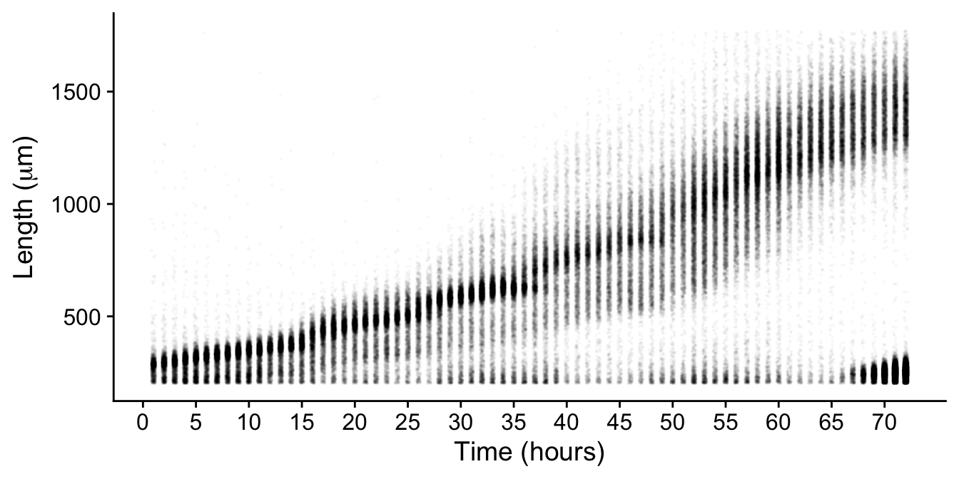
Looking at images its obvious that these are actually the next generation of newly hatched animals!

But how do we selectively remove these from our data without also removing the data we want to keep? I mulled over this question for a while. If I were to simply remove all small objects, I would lose information from the earlier hours of development

filtered <- rawdata %>%
  dplyr::filter(!length < 350)

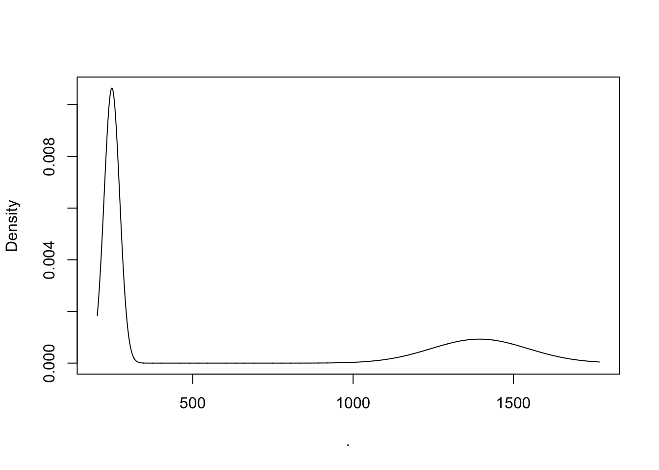
Ideally I would like a way to filter my data on an hour by hour manner without the bias of manually selecting a size threshold. For this I settled on using gaussian finite mixture modeling as implemented in the mclust R package. Specifically, the mclust package fits a mixture model to data and selects the optimal number of clusters using an expectation-maximization algorithm (EM) and Bayes Information Criteria (BIC) – basically it can classify unstructured data into meaningful groups.

H70 <- rawdata %>%
  dplyr::filter(hour == 70) %>%
  dplyr::select(length) %>%
  mclust:: Mclust(., 2)

plot(H70, what = c("density"))

## ---------------------------------------------------- 
## Gaussian finite mixture model fitted by EM algorithm 
## ---------------------------------------------------- 
## 
## Mclust V (univariate, unequal variance) model with 2 components: 
## 
##  log-likelihood    n df       BIC       ICL
##       -32149.42 5450  5 -64341.86 -64343.07
## 
## Clustering table:
##    1    2 
## 3537 1913 
## 
## Mixing probabilities:
##         1         2 
## 0.6489289 0.3510711 
## 
## Means:
##         1         2 
##  247.8094 1394.5085 
## 
## Variances:
##          1          2 
##   591.4166 22783.0510

Alright pretty cool - from the density plot its clear that there are two densities and running mclust shows us how the data was grouped. The smaller cluster of newly hatched animals has an average length of 247.8um and makes up 65% of the data at hour 70.

This would work but to increase the performance of the model-based clustering, I decided to use log transform length and width as inputs.

H70 <- rawdata %>%
  dplyr::filter(hour == 70) %>%
  dplyr::mutate(log.length = log(length),
                log.width = log(width)) %>%
  dplyr::select(log.length, log.width) %>%
  mclust:: Mclust(., 2)

plot(H70, what = c("classification"))

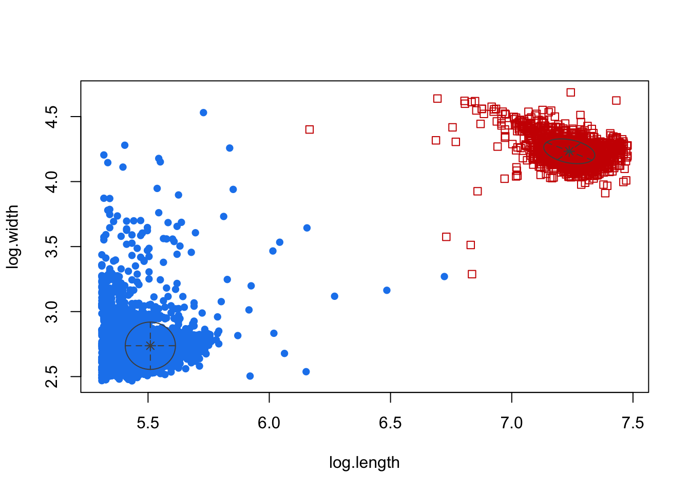There we go! This way it is very clear how the two groups are being classified. Now if we do this across all the hours we can manually select the clusters most likely containing true animals while removing those not.

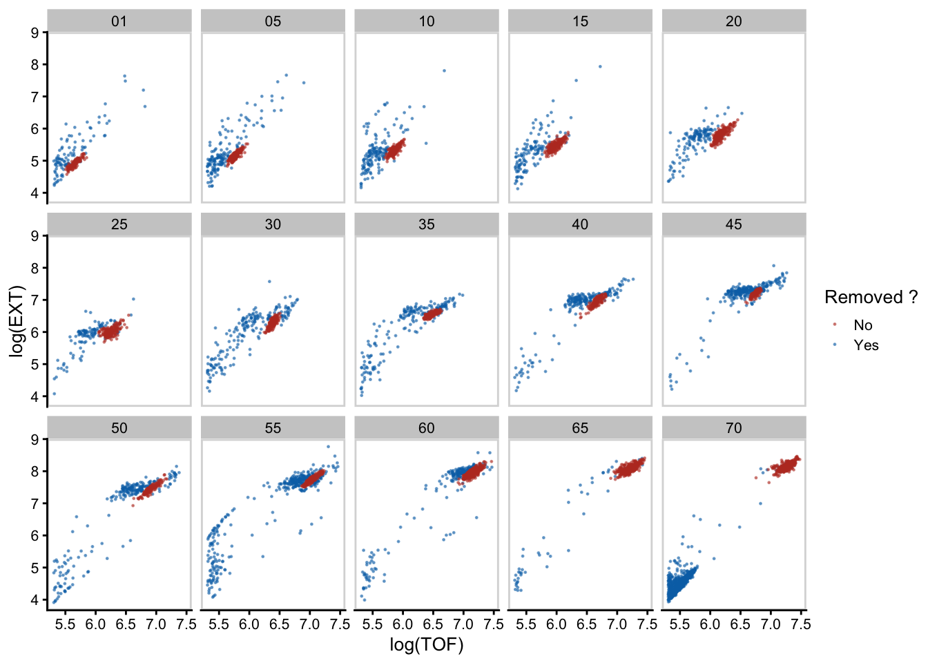
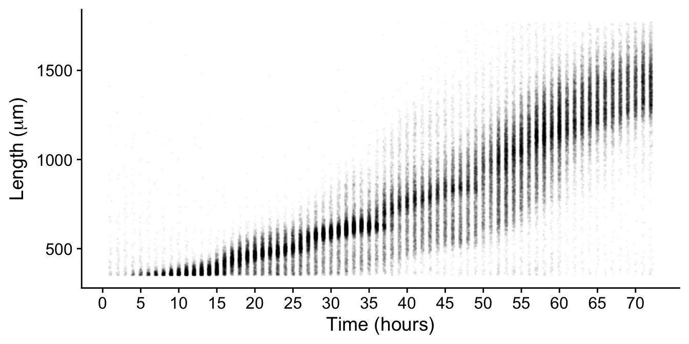
This processing removes non-animal objects such as bacterial clumps, shed cuticles, and next generation larval animals.

total %>%
  ggplot() +
  aes(x = hour, y = TOF, color = `Removed ?`) +
  scale_color_manual(values = c("#BC3C29FF", "#0072B5FF")) +
  geom_jitter(size = 0.3, width = 0.2, alpha = 0.03)+
  scale_x_continuous(breaks = seq(0, 70, 5)) +
  labs(x="Time (hours)", y = expression(paste("Length (", mu,"m)"))) +
  theme_cowplot(font_size = 14, rel_small = 12/14) +  
  guides(color = F)

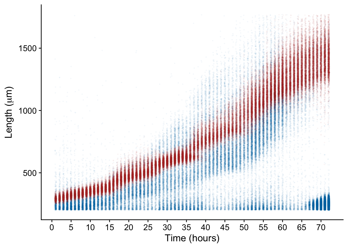
And just like that our data is clean! Now for the fun part – data analysis.