Clustering: Gaussian Mixture Models

Lately, Machine Learning has become such a buzzword in the world of data science. As a biologist, it’s always seemed so daunting… come to find out, it’s really not all that scary!
My first experience in machine learning was with clustering. In my last post I discussed using the mclust package to perform gaussian mixture model (GMM) based clustering on my data. Before I learned of this spectacular package however, I took a stab at implementing my own GMM in R thanks to the help of Fong Chun Chan’s Blog.
Here, I’m just going to go through the fitting of GMM using expectation-maximization (EM) to my worm size data. If you are interested in learning more about GMMs in general I would recommend checking out some of these resources:
“An expectation-maximization algorithm is an iterative method to find local maximum likelihood estimates of parameters in statistical models, where the model depends on unobserved latent variables”
To start, there are 3 steps to this algorithm:
- Initialization
- Expectation (E-step)
- Maximization (M-step)
In order two begin the clustering process, we must first determine what initial model parameters we want to use. The EM algorithm uses the existing data to determine the optimum values for these parameters. Similar to before, I will be looking only at the log transformed data from Hour 70. It is typical to first run k-means on the data to get some initial estimates for model parameters. However, for simplicity I will forgo this step and instead assign the following initial starting parameters.
- Cluster 1: mean = 5.4897, sd = 0.1, pi = 0.7
- Cluster 2: mean = 7.3297, sd = 0.3, pi = 0.3
Now we can move on to step 2: Expectation. Here we need to determine the probability that a data point belongs to a cluster. I like to think of this as a temporary label for each data point.
## dnorm - probability density function for a gaussian distribution
## parameter mu - vector containing mean of each component
## parameter var - vector containing variance of each component
## parameter pi - vector containing probabilities of each component
## function returns a list of loglikelihood values
##  and probabilities for each component

e_step2 <- function(xi,mu.vector,sd.vector,pi.vector) {
  # probability it belongs to cluster 1
  comp1.estep <- dnorm(xi,mu.vector[[1]],sd.vector[[1]]) * pi.vector[[1]]
  # probability it belongs to cluster 2
  comp2.estep <- dnorm(xi,mu.vector[[2]],sd.vector[[2]]) * pi.vector[[2]]
  sum_comps <- comp1.estep + comp2.estep
  # probability it belongs to cluster 1/sum of probabilities
  comp1.post.prob <- comp1.estep/sum_comps
  # probability it belongs to cluster 2/sum of probabilities
  comp2.post.prob <- comp2.estep/sum_comps

  sum_comps_ln <- log(sum_comps,base=exp(1))
  sum_ln_comps <- sum(sum_comps_ln) # loglikelihood value
  list("loglikelihood" = sum_ln_comps,
       "post_prob.df" = cbind(comp1.post.prob, comp2.post.prob))
}
After the E-step comes Maximization. Now that we have temporary assignments for each data point, we need to re-estimate the model parameters that we assigned in step 1.
m_step2 <- function(xi,post_prob.df) {
  comp1.n <- sum(post_prob.df[,1])
  comp2.n <- sum(post_prob.df[,2])

  comp1.mu <- (sum(post_prob.df[,1]*xi)) * 1/comp1.n
  comp2.mu <- (sum(post_prob.df[,2]*xi)) * 1/comp2.n

  comp1.var <- (sum(post_prob.df[,1]*(xi-comp1.mu)^2)) * 1/comp1.n
  comp2.var <- (sum(post_prob.df[,2]*(xi-comp2.mu)^2)) * 1/comp2.n

  comp1.pi <- comp1.n/length(xi)
  comp2.pi <- comp2.n/length(xi)

  # update model parameters
  list("mu" = c(comp1.mu, comp2.mu),
       "var" = c(comp1.var, comp2.var),
       "pi" = c(comp1.pi, comp2.pi))
}
Once we do that we check to see if we have reached reached a point where the change is minimal enough that we can consider it neglible (convergence) at which point we can stop running EM. I am using log likelihood to test for convergence. The main idea being: The larger the log likelihood = The better the fit.
## Returns EM data frame, loglike.vector, likelihood (L), and BIC
## EM df holds parameter values (mu, var, pi) from each iteration (not including initial values)
## loglike.vector holds loglikelihood values from each iteration
## L represents loglikelihood at final iteration
## BIC represents Bayesian Information Criteria at final iteration
EM_alg2 <- function(xi,mu,sd,Pi) {
  # First iteration: Initialize
  estep <- e_step2(xi, mu, sd, Pi)
  mstep2 <<- m_step2(xi, estep[["post_prob.df"]])
  mu1.vector <- mstep2[["mu"]][1] ; mu2.vector <- mstep2[["mu"]][2]
  var1.vector <- mstep2[["var"]][1] ; var2.vector <- mstep2[["var"]][2]
  pi1.vector <- mstep2[["pi"]][1] ; pi2.vector <- mstep2[["pi"]][2]
  current.loglik <- estep[["loglikelihood"]]
  loglike.vector2 <<- estep[["loglikelihood"]]
  repeat {
    # If no longer first iteration: Repeat E and M steps until convergence
    estep <- e_step2(xi, mstep2[["mu"]], sqrt(mstep2[['var']]), mstep2[["pi"]])
    mstep2 <<- m_step2(xi, estep[["post_prob.df"]])
    mu1.vector <- c(mu1.vector, mstep2[["mu"]][1]) ; mu2.vector <- c(mu2.vector, mstep2[["mu"]][2])
    var1.vector <- c(var1.vector, mstep2[["var"]][1]) ; var2.vector <- c(var2.vector, mstep2[["var"]][2])
    pi1.vector <- c(pi1.vector, mstep2[["pi"]][1]) ; pi2.vector <- c(pi2.vector, mstep2[["pi"]][2])
    EM2 <<- cbind(mu1.vector, mu2.vector, var1.vector, var2.vector, pi1.vector, pi2.vector)
    loglike.vector2 <<- c(loglike.vector2, estep[["loglikelihood"]])
    if (estep[["loglikelihood"]] == Inf) {
      break
    }
    loglike.diff2 <<- abs((current.loglik - estep[["loglikelihood"]]))
    if(loglike.diff2 < 10e-6) {
      L2 <<- estep[["loglikelihood"]]
      num <- as.numeric(length(xi))
      BIC2 <<- -2*L2 + 5*log(num)
      break
    } else {
      current.loglik <- estep[["loglikelihood"]]
      next
    }
  }
}
Now to apply this to the data:
mu.H70 <- list(5.4897, 7.3297)
sd.H70 <- list(0.1, 0.3)
pi.H70 <- list(0.7, 0.3)

EM_alg2(H70, mu.H70, sd.H70, pi.H70)
finaldf <- as.data.frame(cbind(tail(EM2,1),BIC2,L2))

plot_mixture <- function(x, mu, sigma, lam) {
  lam * dnorm(x, mu, sigma)
}

rawdata %>%
  dplyr::filter(hour == 70) %>%
  ggplot() +
    geom_histogram(aes(x=log.length, ..density..), binwidth = 0.09, color = "black", fill = "white") +
  stat_function(geom = "line", fun = plot_mixture,
                  args = list(finaldf$mu1.vector, sqrt(finaldf$var1.vector), lam = finaldf$pi1.vector), color = "red", lwd = 1.5) +
  stat_function(geom = "line", fun = plot_mixture,
                  args = list(finaldf$mu2.vector, sqrt(finaldf$var2.vector), lam = finaldf$pi2.vector), color = "blue", lwd = 1.5) +
  theme_bw() + theme(text = element_text(size = 14))
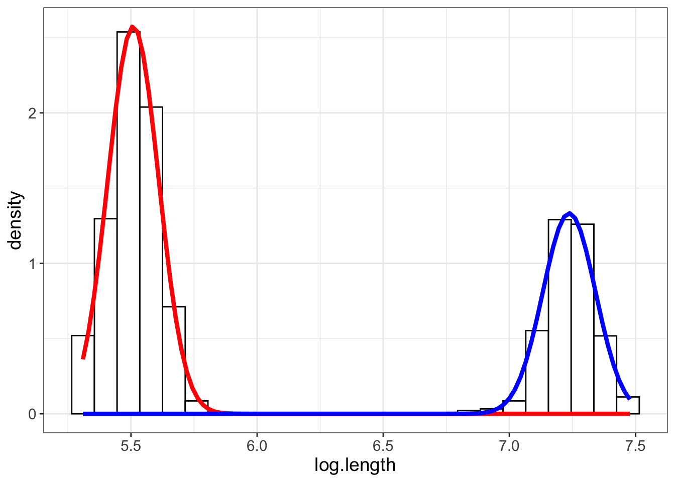
Awesome, it looks like the algorithm did a good job of clustering the data into the visible groups. But of course, I’m curious how this unsophisticated approach compares to the performance of the mclust package.
H70 <- rawdata %>%
  dplyr::filter(hour == 70) %>%
  dplyr::select(log.length) %>%
  mclust:: Mclust(., 2)

# mclust final parameters
H70$parameters
## $pro
## [1] 0.6500917 0.3499083
##
## $mean
##        1        2
## 5.509036 7.237185
##
## $variance
## $variance$modelName
## [1] "E"
##
## $variance$d
## [1] 1
##
## $variance$G
## [1] 2
##
## $variance$sigmasq
## [1] 0.01042731
# our final parameters
tail(EM2,1)
##      mu1.vector mu2.vector var1.vector var2.vector pi1.vector pi2.vector
## [5,]   5.509036   7.237185  0.01014144  0.01095844  0.6500917  0.3499083
Really not too shabby! The final estimated parameters are nearly identical. While this exercise was incredibly useful in understanding how GMM with EM works under the hood, but in application, using a package like mclust provides significantly more information. Biggest takeaway – with the right resources anyone can tackle machine learning!