Analyzing single cell data: Seurat

As promised, this is part 2 of the analyzing single-cell data series. In this post I intend to discuss Seurat: an R toolkit designed for the exploration of single-cell expression data.
Seurat is a well maintained R package that enables users to perform quality control and analysis of single-cell RNA-seq data. Similar to Scanpy's use of AnnData objects, Seurat uses seurat objects as containers for both the count matrix and additional information generated from analyses.
Set Up
library(Seurat)
Again, I will be analyzing the data set of 2,700 single Peripheral Blood Mononuclear cells (PBMC) from 10X genomics. Reading in the data returns a unique molecular identified (UMI) count matrix where rows (i) = genes & columns (p) = cells.
### Read in Data ###
pbmc.data <- Seurat::Read10X(data.dir = "filtered_gene_bc_matrices/hg19")
str(pbmc.data)
## Formal class 'dgCMatrix' [package "Matrix"] with 6 slots
##   ..@ i       : int [1:2286884] 70 166 178 326 363 410 412 492 494 495 ...
##   ..@ p       : int [1:2701] 0 781 2133 3264 4224 4746 5528 6311 7101 7634 ...
##   ..@ Dim     : int [1:2] 32738 2700
##   ..@ Dimnames:List of 2
##   .. ..$ : chr [1:32738] "MIR1302-10" "FAM138A" "OR4F5" "RP11-34P13.7" ...
##   .. ..$ : chr [1:2700] "AAACATACAACCAC-1" "AAACATTGAGCTAC-1" "AAACATTGATCAGC-1" "AAACCGTGCTTCCG-1" ...
##   ..@ x       : num [1:2286884] 1 1 2 1 1 1 1 41 1 1 ...
##   ..@ factors : list()
From here I create the seurat object that will serve as a container that contains both data (count matrix) and analysis.
# Initialize the Seurat object
pbmc <- CreateSeuratObject(counts = pbmc.data, project = "pbmc3k", min.cells = 3, min.features = 200)
pbmc
## An object of class Seurat
## 13714 features across 2700 samples within 1 assay
## Active assay: RNA (13714 features, 0 variable features)
Curious what a count matrix looks like?
# Examine a few genes in the first thirty cells
pbmc.data[c("CD3D", "TCL1A", "MS4A1"), 1:30]
## 3 x 30 sparse Matrix of class "dgCMatrix"
## [[ suppressing 30 column names 'AAACATACAACCAC-1', 'AAACATTGAGCTAC-1', 'AAACATTGATCAGC-1' ... ]]
##
## CD3D  4 . 10 . . 1 2 3 1 . . 2 7 1 . . 1 3 . 2  3 . . . . . 3 4 1 5
## TCL1A . .  . . . . . . 1 . . . . . . . . . . .  . 1 . . . . . . . .
## MS4A1 . 6  . . . . . . 1 1 1 . . . . . . . . . 36 1 2 . . 2 . . . .
the . represents 0s (ie no molecules detected). Seurat uses a sparse=matrix representation
Pre-processing workflow
This workflow involves the selection and filtration of cells based on quality control (QC) metrics, data normalization & scaling, and the detection of highly variable features.
Step 1: QC
I will filter cells based on a few different criteria. These are similar to the metrics used in the Scanpy post.
- Total number of molecules detected within a cell
- Number of unique genes detected per cell
- few genes may indicate low quality cells or empty droplets
- high gene counts may indicate cell doublets or multiplets
- Percentage of reads that map to the mitochondrial genome
- low-quality/dying cells show extensive mitochondiral contamination
pbmc[["percent.mt"]] <- Seurat::PercentageFeatureSet(pbmc, pattern = "^MT-")
# The [[ ]] operator can add columns to object metadata. This is a great place to stash QC stats
Unique genes and total molecules are stored in the object metadata. Here I’ll show the QC metrics for the first 5 cells. I’ll also plot the metrics as a violin plot.
head(pbmc@meta.data, 5)
##                  orig.ident nCount_RNA nFeature_RNA percent.mt
## AAACATACAACCAC-1     pbmc3k       2419          779  3.0177759
## AAACATTGAGCTAC-1     pbmc3k       4903         1352  3.7935958
## AAACATTGATCAGC-1     pbmc3k       3147         1129  0.8897363
## AAACCGTGCTTCCG-1     pbmc3k       2639          960  1.7430845
## AAACCGTGTATGCG-1     pbmc3k        980          521  1.2244898
Seurat::VlnPlot(pbmc, features = c("nFeature_RNA", "nCount_RNA", "percent.mt"), ncol = 3)
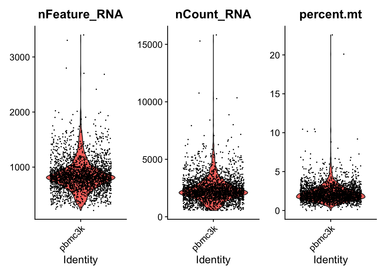
Using this visualization I…
- Filter cells that have unique feature conts > 2500 or < 200
- Filter cells that have > 5% mitochondrial counts
pbmc <- subset(pbmc, subset = nFeature_RNA > 200 & nFeature_RNA < 2500 & percent.mt < 5)
Step 2: Normalizing the data
Now that unwanted cells are removed, the data can be normalized. I will use a global-scaling normalization method “LogNormalize” that (1) normalizes gene expression measurements for each cell by the total expression, (2) multiplies this by a scale factor (10k is default), and (3) log-transforms the result.
pbmc <- Seurat::NormalizeData(pbmc, normalization.method = "LogNormalize")
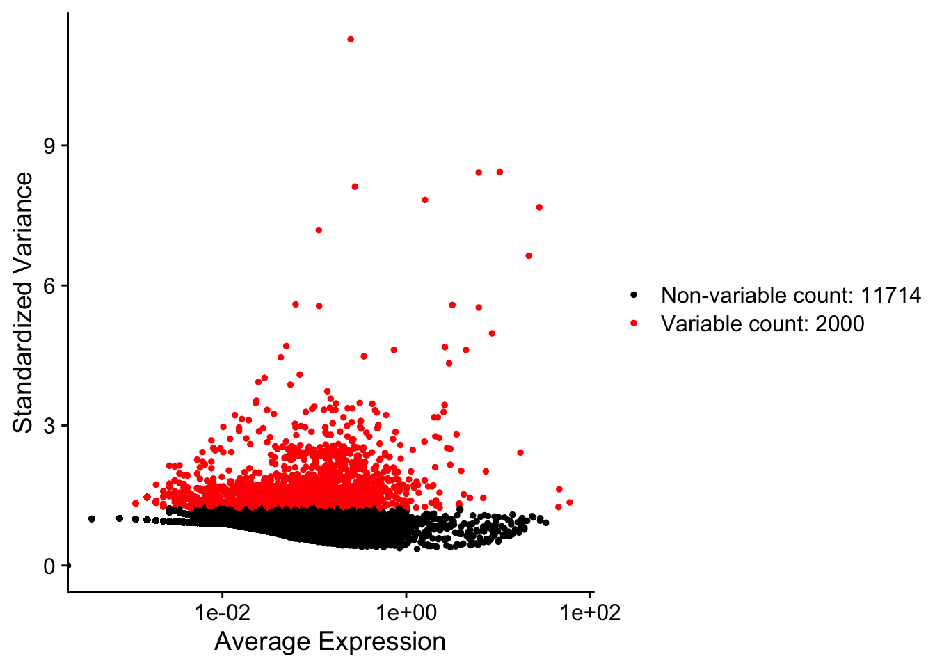
Step 3: Feature Selection
I can then identify a subset of features that exhibit high cell-to-cell variation (HVGs).
pbmc <- Seurat::FindVariableFeatures(pbmc, selection.method = "vst", nfeatures = 2000)

Seurat::VariableFeaturePlot(pbmc)
Step 4: Scaling expression
Finally I rescale the expression of each gene such that mean expression across cells is 0 and variance is 1. This is important so that highly-expressed genes don’t dominate in downstream analyses.
pbmc <- Seurat::ScaleData(pbmc)
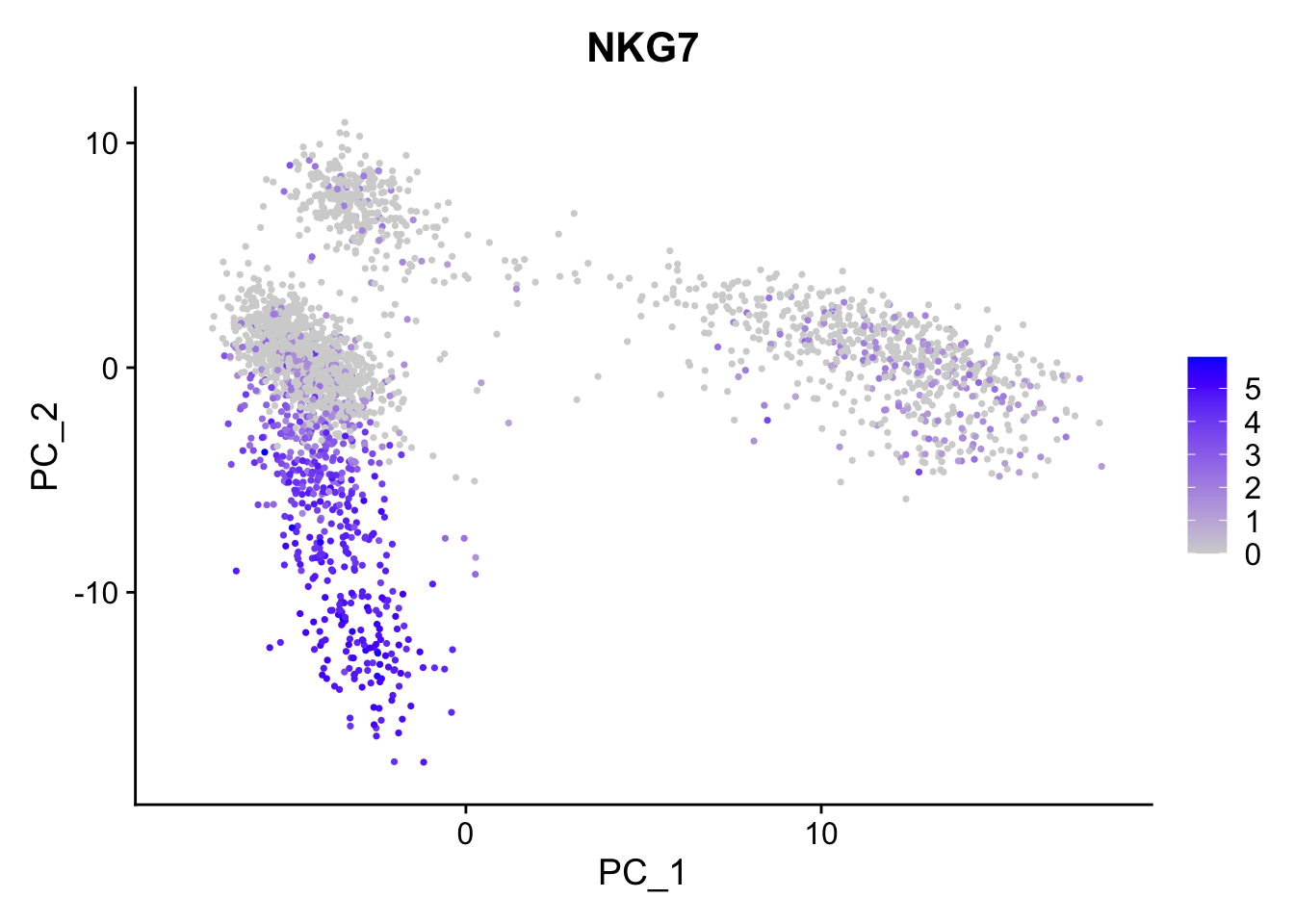
Dimensional Reduction: PCA
Next I perform linear dimensional reduction using only the HVGs.
pbmc <- Seurat::RunPCA(pbmc, features = VariableFeatures(object = pbmc))
Seurat::FeaturePlot(pbmc, features = "NKG7") #show expression of a single gene
Determining dimensionality
An ‘Elbow plot’ can then be used to rank principle components based on the percentage of variance explained by each.
Seurat::ElbowPlot(pbmc)
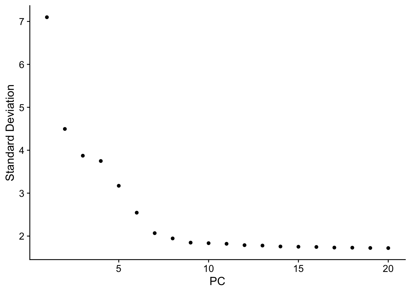
Once again, the first ~10 PCs capture the majority of true signal.
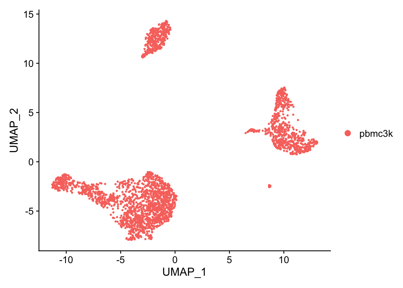
Dimensional reduction: UMAP
Alternatively non-linear dimensional reduction techniques can be used to visualize the data.
pbmc <- Seurat::RunUMAP(pbmc, dims = 1:10)
Seurat::DimPlot(pbmc, reduction = "umap")
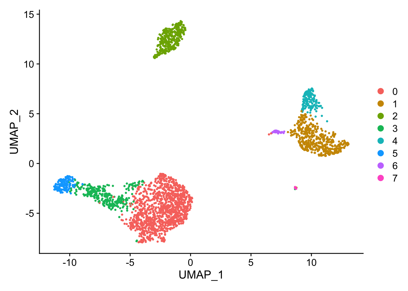
Cluster cells
Now that the data is in a reduced form, I can cluster the cells using the first 10 PCs.
pbmc <- FindNeighbors(pbmc, dims = 1:10)
pbmc <- FindClusters(pbmc, resolution = 0.33)
## Modularity Optimizer version 1.3.0 by Ludo Waltman and Nees Jan van Eck
##
## Number of nodes: 2638
## Number of edges: 95965
##
## Running Louvain algorithm...
## Maximum modularity in 10 random starts: 0.9017
## Number of communities: 8
## Elapsed time: 0 seconds
Seurat::DimPlot(pbmc, reduction = "umap")
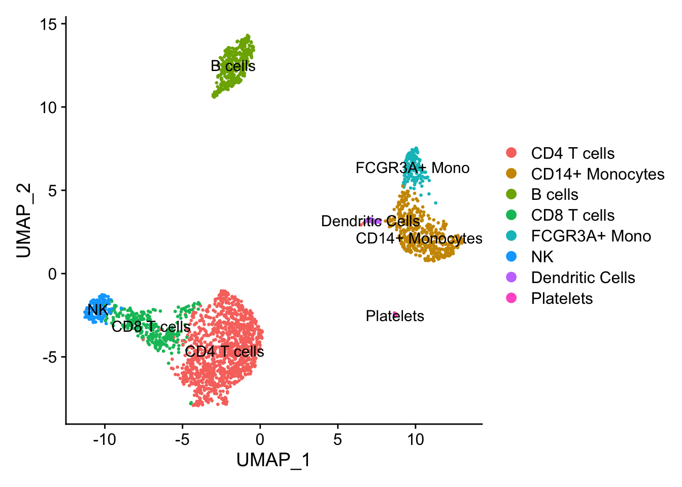
Assign cell type identities to clusters
And finally, I can use canonical markers to match the clusters to known cell types.
new.cluster.ids <- c("CD4 T cells", "CD14+ Monocytes", "B cells", "CD8 T cells", "FCGR3A+ Mono",
    "NK", "Dendritic Cells", "Platelets")
names(new.cluster.ids) <- levels(pbmc)
pbmc <- RenameIdents(pbmc, new.cluster.ids)
Seurat::DimPlot(pbmc, reduction = "umap", label = T, pt.size = 0.5)
 And just like that, we’ve analyzed single cell expression data in both R and python using the
 Seurat and Scanpy packages!